How-to: Data Visualization with External Javascript Libraries (D3 )

One of the great features of Oracle's Business Intellgience 11g foundation is the ability to integrate external applications via an API call or through the use of javascript libraries. In a previous article I discussed how to utilize javascript functions using OBIEE 11g's native UserScripts.js. Today we're going to expand on this functionality by integrating third party data visualization scripts. One popular javascript library used for data manipulation is 'Data-Driven Documents' . This open source scripting library gives users the ability to manipulate data using methods not available in OBIEE 11g.  Kevin McGinley first wrote about this in 2012 and the guys over at Rittman Mead recently posted an overview of D3 / OBIEE integration.  Below we're going to cover all the steps required to implement a D3 visualization technique.

Before we get started, you can view all of the D3 visualization methods at their github. In the example below we're going to use airline data to and D3's Calendar View to visualize average flight delays. You will need OBIEE 11.1.1.6.2 or higher (this example uses OBIEE 11.1.1.7.0) and IE 9+.

 

Step 0: Create an Answers Report

This report should contain a year dimension, a date dimension and an aggregate fact column. In the airline example I've selected 'Date', 'Year' and 'Average Departure Delay'. Take note of the column order as you will have to reference the column number in a narrative.

Step 1: Download the D3 Javascript Library from github

This is going to download a 'd3-master.zip' file that contains all of the javascript libraries needed for integration. You will unzip all of these files into OBIEE 11g's analytics ear deployment under Weblogic's Domain Home  located at :

 user_projects\domains\bifoundation_domain\servers\bi_server1\tmp\_WL_user\analytics_11.1.1\7dezjl\war\res\b_mozilla\common

Step 2:  Create css file for Calendar Formatting

The Calendar view's javascript code is basically one script, with one function and one css file. These 'chunks of code' are all stored in the index.html using the example located on github, but in order for this view to play nice with OBIEE 11g, we're going to need to dissect components of the code into isolated narratives and css files. The first step is to take the css code:

#chart {

  font: 10px sans-serif;

  shape-rendering: crispEdges;

}

.day {

  fill: #fff;

  stroke: #ccc;

}

.month {

  fill: none;

  stroke: #000;

  stroke-width: 2px;

}

and save it to its own css file (calendar.css) located at:

user_projects\domains\bifoundation_domain\servers\bi_server1\tmp\_WL_user\analytics_11.1.1\7dezjl\war\res\b_mozilla\common\d3\examples\calendar\calendar.css (you will need to create the directory as this doesn't exist)

Step 3: Create an Answers Narrative to Execute the Javascript Library

Now that we've laid the groundwork for calling the D3 library, the next step is to integrate the Calendar View code into an Answers narrative.

First create the script headers and link type to call the javascript library. This code will be stored in the pre-fix of the narrative:

<script type="text/javascript" src="/analytics/res/b_mozilla/common/d3/d3.js"></script>

<link type="text/css" rel="stylesheet" href="/analytics/res/b_mozilla/common/d3/lib/colorbrewer/colorbrewer.css"/>

<link type="text/css" rel="stylesheet" href="/analytics/res/b_mozilla/common/d3/examples/calendar/calendar.css"/>

Next we're going to take the calendar view code and copy the entire code block from the start of the width variable delcaration to the end of the call to the selectAll function. Your code should look similar to:

<script type="text/javascript" src="/analytics/res/b_mozilla/common/d3/d3.js"></script>

    <link type="text/css" rel="stylesheet" href="/analytics/res/b_mozilla/common/d3/lib/colorbrewer/colorbrewer.css"/>

    <link type="text/css" rel="stylesheet" href="/analytics/res/b_mozilla/common/d3/examples/calendar/calendar.css"/>

    <div id="my_chart"></div>

    <script type="text/javascript">

var margin = {top: 19, right: 20, bottom: 20, left: 19},

    width = 720- margin.right - margin.left, // width

    height = 136 - margin.top - margin.bottom, // height

    cellSize = 12; // cell size

var day = d3.time.format("%w"),

    week = d3.time.format("%U"),

    percent = d3.format(".1%"),

    format = d3.time.format("%Y-%m-%d");

var color = d3.scale.quantize()

    .domain([5,30])

    .range(d3.range(9));

var svg = d3.select("#my_chart").selectAll("svg")

    .data(d3.range(year_range1, year_range2))

  .enter().append("svg")

    .attr("width", width + margin.right + margin.left)

    .attr("height", height + margin.top + margin.bottom)

    .attr("class", "RdYlGn")

  .append("g")

    .attr("transform", "translate(" + (margin.left + (width - cellSize * 53) / 2) + "," + (margin.top + (height - cellSize * 7) / 2) + ")");

svg.append("text")

    .attr("transform", "translate(-6," + cellSize * 3.5 + ")rotate(-90)")

    .attr("text-anchor", "middle")

    .text(String);

var rect = svg.selectAll("rect.day")

    .data(function(d) { return d3.time.days(new Date(d, 0, 1), new Date(d + 1, 0, 1)); })

  .enter().append("rect")

    .attr("class", "day")

    .attr("width", cellSize)

    .attr("height", cellSize)

    .attr("x", function(d) { return week(d) * cellSize; })

    .attr("y", function(d) { return day(d) * cellSize; })

    .datum(format);

rect.append("title")

    .text(function(d) { return d; });

svg.selectAll("path.month")

    .data(function(d) { return d3.time.months(new Date(d, 0, 1), new Date(d + 1, 0, 1)); })

  .enter().append("path")

    .attr("class", "month")

    .attr("d", monthPath);

    var csv =[];

Notes About this Code

Although this code does most of the heavily lifting and can be left unmodified, there are specific lines that can be changed and updated dynamically via the use of presentation variables.

Color Thresholds:

The color variable specifies the thresholds for red/yellow/green. In this case I deem the min and max ranges of an airline delay to be between 5 minutes and 30 minutes:

var color = d3.scale.quantize()

    .domain([5,30])

Chart Size Adjustment:

By modifying the code for the margin variable:

var margin = {top: 19, right: 20, bottom: 20, left: 19},

    width = 720- margin.right - margin.left, // width

    height = 136 - margin.top - margin.bottom, // height

    cellSize = 12; // cell size

  The height/width/cell size can be adjustable by changing the hardcoded values to presentation variables such as:

• @{Width}
• @{Height}
• @{CellSize}

Date Formatting:

The 'day' variable responsible for date formatting:

var day = d3.time.format("%w"),

    week = d3.time.format("%U"),

    percent = d3.format(".1%"),

    format = d3.time.format("%Y-%m-%d");

Requires that the format of the date be specified.  The Calendar View script by default uses a 'YYYY-MM-DD' format. If your OBIEE data is a MM-YY-DD format or has a timestamp, you will need to modify the column data format to the following:

Modifying the Date Range:

The Calendar View code by default hard codes a date range of 1990 to 2011. You will most likely need to modify these values for your data set create a presentation variable that allows the users to change the date range dynamically:

var svg = d3.select("body").selectAll("svg")
    .data(d3.range(1990, 2011))

Could be modified to:

var svg = d3.select("#my_chart").selectAll("svg")
    .data(d3.range(year_range1, year_range2))

In the upcoming steps I will show how these variables can be called.

 Step 4: Populate the Narrative and Post-Fix

In the narrative you will need to specify the Date and Metric you want to pass to the javascript function using the corresponding column number (see step 0 if you forgot!)

The Post-Fix should contain the remainder of the Calendar View code. This can remain unmodified:

var data = d3.nest()
    .key(function(d) { return d.Date; })
    .rollup(function(d) { return d[0].Metric; })
    .map(csv);
  rect.filter(function(d) { return d in data; })
      .attr("class", function(d) { return "day q" + color(data[d]) + "-9"; })
    .select("title")
      .text(function(d) { return d + ": " + (data[d]); });
function monthPath(t0) {
  var t1 = new Date(t0.getFullYear(), t0.getMonth() + 1, 0),
      d0 = +day(t0), w0 = +week(t0),
      d1 = +day(t1), w1 = +week(t1);
  return "M" + (w0 + 1) * cellSize + "," + d0 * cellSize
      + "H" + w0 * cellSize + "V" + 7 * cellSize
      + "H" + w1 * cellSize + "V" + (d1 + 1) * cellSize
      + "H" + (w1 + 1) * cellSize + "V" + 0
      + "H" + (w0 + 1) * cellSize + "Z";
}
</script>

Your narrative should be similar to:

Step 5: Create a Second Narrative for the Date Range

This narrative is optional, but assuming you want to give the user the ability to modify the date range, you would take the variables you referenced in the 'Modifying the Date Range' section (in my case year_range1 and year_range2)  and set both of them equal to two presentation variables like below:

Step 6: View Narratives in Answers

Adding both narratives to a single view, your end result should look similar to:

This guide barely scratches the surface of D3-OBIEE integration but serves as a great example of how 3rd party APIs and javascript libraries can be integrated into OBIEE 11g. I encourage all BI Architects to look through the entire D3 library and see how D3 can be integrated into their current engagement.

 

 keywords: OBIEE 11g, Data-Driven Documents, OBIEE 11.1.1.7.0, UserScripts.js, Answers, javascript

Overview on Object Level Security, Application Roles, and Inheritance in OBIEE 11g

In Oracle Business Intelligence (OBIEE) 11g, Oracle has fundamentally changed how we map users to various security privileges.In OBIEE 10g, Object Level Security was enforced using the USER session variable, which mapped to a GROUP session variable. This created a list of possible 'groups', which a developer would then apply security restrictions to, in either Answers (Managed Privileges) and/or Security Managed in the repository.

A high level flow is outlined below:

In OBIEE 11g, security authentication is enforced in the Weblogic Admin Server, and a user's security privileges are tied to their corresponding Application Roles in Fusion Middleware as shown in the diagram below:

The key take away is that object level security is applied to application roles and not groups.  Why application roles? In Weblogic and Fusion Middleware, we can actually assign certain privileges to an application roles - we call these 'Application Policies'. For example,  we can grant a certain application role the ability to 'edit the repository', or 'act as another user'. This feature, not possible in OBIEE 10g, now allows us to not only control what objects are being viewed, but also gives us the capability to control who can execute certain actions within the BI environment. This topic will be discussed in much greater detail in another guide.

Now let's go over the basic rules of Object Level Security for Application Roles in OBIEE 11g:

• If a user is a direct member of an application role, they will have access to the reports allowed by that application role.
• If a user is not a member of an application role, they will not have access to the reports allowed by that application role.
• If a user is a direct member of two or more application roles with different security privileges for the same reports, the less restrictive security privilege is applied.
• unless the user is explicitly denied. Explicit denial supersedes all security privileges.
• If a user is a member of Application Role X, and Application Role X is a member of Application Role Y, the privileges in Application Role X supersede the privileges of Application Role Y

Let's cover each scenario in detail:

• If a user is a direct member of an application role, they will have access to the reports allowed by that application role.

 

In this example, I granted Application Role 'Test Role 1' full control to folder 'Folder 1'. I then logged in as 'testuser1' who is a member of Application Role 'Test Role 1'. And as expected, testuser1 can read/write/edit/delete the folder.

• If a user is not a member of an application role, they will not have access to the reports allowed by that application role.

In this example, I created 'Folder 2', only accessible by members of the 'BIAdministrator Application Role'. I then log in as a 'testuser1', which is not a member of the 'BIAdministrator Application Role'

As BIAdministrator:

As testuser1:

Note that in the above scenario, 'denying' the application role access accomplishes the same thing as taking no action onto the application role role (i.e. ignoring it completely)

• If a user is a direct member of two or more application roles with different security privileges for the same reports, the less restrictive security privilege is applied.

In this example, I created Folder 3, which grants 'read' access to Test Role 1 and 'modify' access to 'Test Role 2'. 'Testuser1' is a member of both 'Test Role 1' and 'Test Role 2'.

 

 

As expected, Testuser1 has modify rights to Folder 3 (noted by 'X', ability to delete), despite being a member of Test Role 1 which only grants the user read access

• If a user is a direct member of two or more application roles with different security privileges for the same reports, the less restrictive security privilege is applied.
• unless the role is explicitly denied

In this example, TestUser1 is a member of Test Role 1 and Test Role 2 and Test Role 3. Test Role 1 grants testuser1 open rights, Test Role 2 grants testuser1 modify rights and Test Role 3 is explicitly denied.

As expected, testuser1 does not have access to Folder 4 because of Test Role 3

• If a user is a member of Application Role X, and Application Role X is a member of Application Role Y, the privileges in Application Role X supersede the privileges of Application Role Y

 

In this example, testuser1 is a member of application role 'Test Role 4'. Application role 'Test Role 5' is a member of application Role 'Test Role 4'. Test Role 4 grants 'open' privileges to Folder 5 and Test Role 5 grants 'full control' to Folder 5.

 

As expected, testuser1 only has read/open access to Folder 5 even though Application Role 'Test Role 5' grants full control. This is because direct inheritance overrides indirect inheritance

Even if the inherited role explicitly denies access to folder 5, the user will still be able to access folder 5 because the direct role grants read/open access:

Note how testuser1 has modify access to Folder 5 (noted by the 'X') , despite inheriting a role that is denied access to the same folder.

These basic rules can be applied to any hierarchy, no matter how complex. Think you've mastered these 4 basic rules? Identify the final privileges for User 1 in the scenario below:

* example courtesy of Oracle - found in Oracle Business Intelligence Fusion Middleware Security Guide

Result:

• User is a direct member of Role 1 and 2 and indirect member of Role 3, Role 4 and Role 5
• User has no access to Dashboard A
• User has open access to Dashboard B
• User has full control of Dashboard C
• User has no access to Dashboard E
• User has open access to Dashboard D

 keywords : object level security, obiee security, obiee application roles, obiee 11g security, weblogic application roles, obiee inheritance

How-to: OBIEE 11g Javascript Integration using Action Framework (Browser Script)

One of the powerful features of Oracle's Business Intelligence 11g platform is a concept called 'Action Framework' or 'Actionable Intelligence'. It's useful because for the first time in OBIEE you can integrate external applications, functions or code and invoke it using the front end user interface (Answers).

Although I have seen 'javascript or jquery integration' in OBIEE 10g, the implementation was always 'hacked' together, and of course, was never supported or endorsed by Oracle. In this guide we'll show how you can take any javascript or jquery function and by using Oracle's supported 'external systems framework', integrate it seamlessly with OBIEE 11g.

Consider the scenario where your source data warehouse or ERP stores employee numbers in an encoded format of base 64. For example, employee number '123456789' is 'MTIzNDU2Nzg5' in base 64.  The requirement you have is to display the decoded employee number in a report. How do we implement this requirement?

Luckily, base 64 encode/decode functions are easily accessible via the internet, so we'll use the code from Stackoverflow.com

The encode function will ultimately end up in the UserScripts.js file located at:

• <middleware home>/user_projects/domains/bifoundation_domain/servers/bi_server1/tmp/_WL_user/analytics_11.1.1.2.0/<installation dependent folder>/war/res/b_mozilla/actions/UserScripts.js

But we can't just copy & paste, so let's get started.

Step 1: Understand how OBIEE 11g uses action framework to invoke custom javascript functions

OBIEE 11g stores custom javascript functions in Userscripts.js. In order to integrate a javascript function into userscript.js your function  must have:

• a USERSCRIPT.publish function which is required to pass the parameters to the target javascript function
• a USERSCRIPT.parameter function out of the box function which is used by the Action Framework to define parameters in custom JavaScript functions for use when creating an action to Invoke a Browser Script. Each parameter object includes a name, a prompt value holding the text to be displayed against the parameter when creating an action, and a default value.
• a USERSCRIPT.encode function - the actual function we're going to implement

Step 2: Create USERSCRIPT.encode.publish function


As described above, the userscript.encode.publish function needs to take the parameters from the USERSCRIPT.parameter file and create a new encode object:

USERSCRIPT.encode.publish=
{
 parameters:
 [
  new USERSCRIPT.parameter("employeenumber","Employee Number","")
 ]
}

 Step 3: Create the actual encode functions

The encode function from stackoverflow is actually comprised of two functions: 1) the public method for encoding and 2) the private method used for UTF8 encoding

USERSCRIPT.encode function:

USERSCRIPT.encode=function(b)
{
var cz="";
for(args in b)
 { // this for function is needed to store the 3rd value in the array - the actual employee number
 var d=args;
 var a=b[d];
 cz = a;
 }
 var output = "";  
 var chr1, chr2, chr3, enc1, enc2, enc3, enc4;
 var i = 0;
 var _keyStr = "ABCDEFGHIJKLMNOPQRSTUVWXYZabcdefghijklmnopqrstuvwxyz0123456789+/=";
 var input = USERSCRIPT.UTF8Encode(cz);

 while (i < input.length)
 {

  chr1 = input.charCodeAt(i++);
  chr2 = input.charCodeAt(i++);
  chr3 = input.charCodeAt(i++);

  enc1 = chr1 >> 2;
  enc2 = ((chr1 & 3) << 4) | (chr2 >> 4);
  enc3 = ((chr2 & 15) << 2) | (chr3 >> 6);
  enc4 = chr3 & 63;

  if (isNaN(chr2)) {
   enc3 = enc4 = 64;
  } else if (isNaN(chr3)) {
   enc4 = 64;
  }


  output = output +
  _keyStr.charAt(enc1) + _keyStr.charAt(enc2) +
  _keyStr.charAt(enc3) + _keyStr.charAt(enc4);
 }

alert(output)
}
;

USERSCRIPT.UTF8ENCODE function

USERSCRIPT.UTF8Encode=function(b)
{   
 var str = b.replace(/\r\n/g,"\n");   
 var str = b;

 var utftext = "";
 for (var n = 0; n < str.length; n++) {
  var c = str.charCodeAt(n);
  if (c < 128)
  {
   utftext += String.fromCharCode(c);
  } else if((c > 127) && (c < 2048)) {
   utftext += String.fromCharCode((c >> 6) | 192);
   utftext += String.fromCharCode((c & 63) | 128);
  } else {
   utftext += String.fromCharCode((c >> 12) | 224);
   utftext += String.fromCharCode(((c >> 6) & 63) | 128);
   utftext += String.fromCharCode((c & 63) | 128);
  }
 }

 return utftext;
 };

After this, make sure to restart Admin Service, Managed Server and OPMN prior to creating the Action in Answers

Step 4: Create the Action in Answers

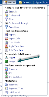
In Answers, navigate to New -> Actionable Intelligence -> Action -> Invoke -> Invoke a Browser Script

1) 2)

Click browse and select the USERSCRIPT.encode function:

Since the USERSCRIPT.parameter function specified 3 parameters, we will need to populate the three fields  as follows: Object Name, prompt value, and default value.

After saving the action, execute it and populate it with a number, or leave it as default 123456789.

And as expected, the encoded base 64 number 123456789 is - 'MTIzNDU2Nzg5'

This example only scratches the surface of what's possible with Action Framework and OBIEE 11g. Correctly implemented, you can invoke 3rd party applications or functions (*cough* ETL on demand *cough*), pass data to the ERP source system, integrate a data set with Google Maps, or all of the above.

In future guides we will explain the advanced functionality of Action Framework.

 keywords: action framework,  obiee action framework, obiee javascript, obiee actions,  actionable intelligence

How-to: Image Referencing with OBIEE 11g

In a typical OBIEE engagement, the client may want to utilize out of the box or custom images within various dashboards and reports. This requirement leads to many open questions, including:

1. Where are these images located?
2. How do I embed the image into a dashboard or report?
3. How do I maintain the integrity of the image URL across multiple environments?

Let's break down each question one by one:

Where are these images located?

All images are stored in the 'browser look and feel plus' folder of the BI Server, you've probably seen this notated as 's_bflap'. This folder exists in two locations and it is critical that any image you upload be housed in both:

• Oracle_BI1\bifoundation\web\app\res\s_blafp\images
• user_projects\domains\bifoundation_domain\servers\bi_server1\tmp\_WL_user\analytics_11.1.1\7dezjl\war\res\s_blafp\images

How do I embed the image into a dashboard or report?

OBIEE 11g has a little known feature called 'fmap' which can be used to display an image based on the relative URL of the image. Little documentation exists on it other than a few notes released by Oracle which include:

• How To Display Custom Images Using Fmap In OBIEE 11g (Doc ID 1352485.1)
• Image FMAP on Linux (Doc ID 491154.1)

How do I maintain the intregrity of the image URL across multiple environments?

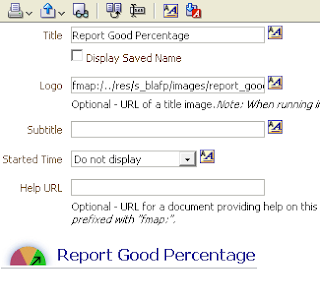
Here is where things get tricky due to the lack of documentation that exists.  Let's say you want to use the image 'report_good_percentage.jpg' located in the s_blafp folder:

So as outlined in Oracle's documentation you use 'fmap:report_good_percentage.jpg' or even 'fmap:images/report_good_percentage.jpg', but to your dismay all you see is a broken image link:

Why?

It is important to remember that fmap displays the image of the relative URL. So what does relative mean? What is 'it' relative to? In regards to fmap, the relative URL is the root directory of the analytics web server, which in OBIEE 11g is:

/export/obiee/11g/user_projects/domains/bifoundation_domain/servers/bi_server1/tmp/_WL_user/analytics_11.1.1/7dezjl/war

Which makes sense if you understand how applications are deployed in weblogic. The presence of the WEB-INF directory in the aforementioned folder is how Weblogic determines if a folder if a deployable application directory.

So - if we work under the assumption that the above folder is indeed the root directory, then it we now know why the image returns a broken link, report_good_percentange.jpg is not stored in the 'root' directory of the analytics web server, it is actually stored in:

/export/obiee/11g/user_projects/domains/bifoundation_domain/servers/bi_server1/tmp/_WL_user/analytics_11.1.1/7dezjl/war/res/s_blafp/images

Let's update the fmap relative url to correctly reference report_good_percentage.jpg by modifying it to:

fmap:res/s_blafp/images/report_good_percentage.jpg

Unfortunately..

Why does fmap STILL not work?

Let's take a look at the URL that's actually being generated:

Notice anything funny? Why is OBIEE 11g adding a 'Missing_' folder to the URL directory? Countless bloggers have theorized this as a bug in OBIEE and some even suggest making a 'Missing_' folder in the root directory of the analytics web server. I don't think that is the best approach because as you deploy this application across multiple servers, you'll have to make sure all environments have that same folder. Keep it simple right?

We can resolve this by modifying the fmap url to revert one directory closer to its root by using '/..':

fmap:/../res/s_blafp/images/report_good_percentage.jpg

Let's check the URL being generated just to make sure:

 The image displays, and the 'Missing_' folder is no where to be found.  If your requirements have extensive image customizations, perhaps changing the entire look and feel, I recommend deploying an entirely new skin as outlined in Oracle Note: How to Use Custom Images in OBIEE (Doc ID 1484623.1)

How-to: Mapviewer Integration with OBIEE 11g (11.1.1.6 and higher)

I've seen quite a few articles on OTN and Google which outline how to configure Mapviewer for your 11g solution.  The problem is that many of these articles are:

1) overly complex
2) out of date

With the release of OBIEE 11.1.1.6, mapviewer comes pre-configured with weblogic and the only installation steps required are:

• installation of navteq mapdata to your oracle database
• establish a column based relationship between the map and a subject area

You do not have to modify any weblogic XML files, install any mapviewer jar files, or do any configuration within weblogic. Below is a step by step guide on how to configure and use mapviewer on your 11.1.1.6.x box:

Step 1: Download the mapviewer 'mvdemo' data into your Oracle database

Oracle provides pre-configured maps, coordinates, and navteq data that use can use in your reports. You need to download the MVDemo Sample Data Set .

Step 2: Create the mvdemo schema in your Oracle database

We're going to import the navteq map data into an mvdemo schema in step 3. Let's go ahead and create the mvdemo schema by typing the following command into your SQLPlus prompt:

grant connect, resource, create view to mvdemo identified by mvdemo

Note that you will need the appropriate privileges to create this account. If denied, try logging in as sysdba by typing the following command into sqplus:

CONNECT / AS sysdba

Step 3: Import navteq data dump to your Oracle database

Unzip the MV Demo Sample Data Set you just downloaded, and note the location of the 'mvdemp.dmp' file. This is the file we will import to the database.


Step 3.1)
Find the imp utility on your machine. It is usually located in your $ORACLE_HOME\product\11.x.x\dbhome_1\BIN folder

Step 3.2) Navigate to that folder via command line and run the following command:

imp mvdemo/mvdemo@ORCL file=mvdemo.dmp full=y ignore=y
where ORCL is your database SID
and file=mvdemo.dmp is the path (including mvdemo.dmp) to the dump file

You should get the following result:

Step 4) Import the map meta data

The Map Viewer Sample Data Set comes with city, county, state, highway, and other geographical map based data that you can impose onto the map. We're going to import this data set by running the following command in sqlplus:
:
@mvdemo.sql

Note that you must include the path of the mvdemo.sql file e.g. @C:\folder\folder1\mvdemo\mvdemo.sql

Step 5) Add your Oracle Database as a MapViewer Data Source

No, we're not doing this in weblogic - Mapviewer data source configuration is still done in your http://localhost:9704/mapviewer location


You'll arrive at a landing page like below, where you must click the 'Admin' button to log in:

5.1) login user your weblogic username/password

5.2) You should arrive at a home page with a link to view Datasources. Click it and you'll appear at:

Name = name/description of your data source

Host = hostname/ip address of your database

Port = database port number

SID = service ID of your oracle database (by default it is orcl)

user/password: If you followed my above steps, it will be mvdemo/mvdemo

# Mappers and Max Connections specify how many simultaneous users can connect to the MapViewer db. For diagnostic purposes I would make this relatively high, and once development is complete you can adjust as needed.

Step 6) Modify the mapViewerConfig.xml file to include the new data source

I'm a little surprised as to why this must be done manually, if anyone has any insight - please feel free to leave feedback. After you add the data source as outlined in step 5, you must then modify the mapViewerConfig.XML file to include said datasource, otherwise when the BI Server is rebooted, your datasource connection will be removed!

Luckily, this step is not too difficult

6.1) In :7001/mapviewer , log into your Admin screen and navigate to Management -> Configuration

Then add the following XML to the bottom of the config file, right above the </MappperConfig> line.

  <map_data_source name="mvdemo"

                   jdbc_host="db1.my_corp.com"

                   jdbc_sid="orcl"

                   jdbc_port="1521"

                   jdbc_user="scott"

                   jdbc_password="!tiger" 

                   jdbc_mode="thin"

                   number_of_mappers="3"

                   allow_jdbc_theme_based_foi="false"

   />

Modify each line using the inputs you provided in step 5, but in the jdbc_password input should have a ! infront of it as that is Oracle's indicator to encrypt the password upon restart.

Step 7)  Import a map layer into Answers 

We've completed all of the back end work required to create a map. Now we'll go into Answers -> Administration -> Manage Map Data and import a layer (theme) that we'll use for our map.

A theme is a visual representation representation of the data, and arguably the most important component in creating a map. In this example let's use the "THEME_DEMO_COUNTIES" layer, which will give us the ability to impose a dataset over various Counties in the USA.

Step 8) Specify the BI Column used to associate the THEME_DEMO_COUNTIES layer to a dataset

The theme we're using, "THEME_DEMO_COUNTIES" stores attributes of Counties (county name, county lines, etc) which we can visualize on a map. We need to identify a way to 'join' the data set in OBIEE to the dataset of THEME_DEMO_COUNTIES.

After saving the layer you just created, click the 'Edit' button (pencil) to bring up the screen below.

Notice there is 'Layer Key' with the following column values; County, Fips, Population, State.  We are going to use 'County' as the map column to join to the subject area.

Next we need to specify a column from our subject area which contains 'County'.  

Step 9) Specify the Background Map

In steps 7 and 8 we specified a theme (visual representation of the data) and identified how to join the map data to our subject area (via County column). Now we need to specify which map we're the theme will use.

In the 'Background' tab, create a new background map and specify 'DEMO_MAP' as the background map.

After saving, edit the map ensure the THEME_DEMO_COUNTIES has successfully been applied:

It will default to the middle of the USA but I decided to zoom into California :)

Step 10) Create a Report using the County Column 

Now we're ready to create the report! Create a new analysis, select the County column you specified in step 7, and a fact column which joins to the county dimension. Click the results tab, then New View -> Maps.  

The result below outlines only California because the dataset I created uses only California Counties. 

Note that I did not go into the MapBuilder tool, which you can use if you want to create custom themes and maps (e.g. map of a building, school, casino, etc). But this works great for a proof of concept!

 keywords: obiee mapviewer, rendering maps, obiee configuration, obiee 11g maps, obiee navteq maps, obiee mapviewer integration

How-to: Bridge Tables and Many to Many Relationships Demystified in OBIEE 11g

Bridge tables - entire books have been devoted to this concept, countless blogs write about it, and organizations offer entire classes dedicated to demystifying this idea. Ralph Kimball, creator of Kimball Dimensional Modeling and founder of the Kimball Group has written quite a few great articles discussing the theory of bridge tables.

Yet when researching for comprehensive guides on how to actually implement a bridge table in OBIEE 11g, the documentation available is either:

• Out of date
• Contains implementation steps for OBIEE 10g which has since been deprecated
• Does not contain adequate detail 
• e.g. missing key steps

This guide is going to outline the basic use case of a many to many relationship, how OBIEE 11g resolves this dilemma and how to successfully implement a bridge table model within the 11g platform.

First thing's first - what is a bridge table and why do we need it?

At its core, bridge table solve the many to many relationship we encounter in many datasets. Many to many relationships in itself are not "bad", but when attempting to conform a data set to a star schema - many to many relationships just do not work. Star schemas assume a one to many (1:N) cardinality from the dimension to the fact. This means "one attribute of a dimension row can be found in many rows of the fact table".

For Example:

• One job (job dimension) can be performed by many people
• You would see the same JOB_WID repeating in the fact table
• One employee (employee dimension) can have many jobs
• You would see the same EMPLOYEE_WID  repeating in the fact table
• One call at a call center(ticket dimension) can have many ticket types
• You would see the same CALL_WID repeating in the fact table
• One patient (patient dimension) can have many diagnosis
• You would see the same PATIENT_WID repeating in the fact table

This 1:N cardinality is represented in OBIEE as (using call center/employee example) :

"Cardinality of '1' applied to the dimension and cardinality of 'N' applied to the fact'

But what happens when in the above examples, the cardinality is actually N:N? 

For Example:

• Many employees can have multiple jobs and each job can be performed by multiple employees
• Many patients can have multiple diagnosis and each diagnosis can be 'assigned' to many patients
• Many calls can have multiple call ticket types and each ticket type can belong to multiple calls

This many to many relationship is initially (and incorrectly) represented in OBIEE 11g as:

'Cardinality of '1' is applied to the two dimension tables and cardinality of 'N' is applied to the fact'

Any BI Architect should recognize the above model - it's a traditional star schema! If you stop here and decided to ignore the issue with your dataset and 'hope' OBIEE aggregates the model correctly, you're about to be disappointed.

Why star schemas dont work for N:N cardinality

Consider the following scenario: You're a call center manager and you want to capture the number of calls with positive feedback per employee. You also want to capture the type of calls an employee answers in any given day.

Upon analysis of the requirements you conclude that "each call received by an employee can have many call types and each call type can be answered by multiple employees".

For example:

• I answer a take a call that is classified as a 'new call', 'urgent', and 'out of state transfer' (three different call types) - this is the "each call received by an employee can have many call types".
• A colleague also received a phone call that is classified as 'out of state transfer' - this is the 'each call type can be answered by multiple employees"

Now let's put this data in a traditional star schema fact table as modeled below:

ID	EMPLOYEE_WID	CALL_TYPE_WID	NUMBER_OF_GOOD_CALLS
1	1	1	300
2	1	2	300
3	1	3	300
4	2	2	500
5	2	3	500
6	3	1	200

You can see in the above data set that:

• EMPLOYEE 1:
• Has 3 different call types
• Has 300 positive reviews (NUMBER_OF_GOOD_CALLS) 
• This metric is at the EMPLOYEE level and not the call type level!
• EMPLOYEE 2:
• Has 2 different call types
• Has 500 positive reviews (NUMBER_OF_GOOD_CALLS)
• This metric is at the EMPLOYEE level and not the call type level
• EMPLOYEE 3:
• Has 1 different call type
• Has 200 positive reviews (NUMBER_OF_GOOD_CALLS)

Now you receive a requirement to create a KPI that displays the Number of Good Calls as a stand alone widget.

PROBLEM 1 - Aggregation :

The number of good calls you received based on the above fact table is not 2100 - it's 300 + 500 + 200 = 1000

• Employee 1 received 300 good calls
• Employee 2 received 500 good calls
• Employee 3 received 200 good calls

but due to the many to many cardinality of the data, the star schema duplicates the measures because each employee can take calls of many call types and each call type can be assigned to many employees!

PROBLEM 2 - Grand Totaling:

What if you don't care about aggregates? What if you just want a report that contains the employee, call type and a summation/grand total?

Notice how NUMBER_OF_GOOD_CALLS is repeated across multiple call types and the grand total is still incorrect. It's being duplicated due to the many to many relationship that exists between call type and employee. Furthermore, it paints an incorrect picture that NUMBER_OF_GOOD_CALLS is some how related to CALL_TYPE

How do we resolve this many to many cardinality with a bridge table?

When all is said and done, the incorrectly built star schema:

should be modified to:

Let's break this down:

The bridge table:

This the purpose of the bridge table is to resolve the many to many relationship between the call type and employee. It will contain, at a minimum, the following four columns:

1. The primary key of the table
2. The EMPLOYEE_WID
3. The CALLTYPE_WID
4. The weight factor

The weight factor is what's going to resolve the issue of double counting. 

• If an employee has 3 call types, there would be 3 rows and the weight factor of each row would be .33
• If an employee has 10 call types, there would be 10 rows and the weight factor of each row would be .1

In our bridge table data set, we're going to use the same 3 EMPLOYEE_WIDs and create the following:

ID	CALL_TYPE_WID	EMPLOYEE_WID	WEIGHT
11	1	1	0.33
12	2	1	0.33
13	3	1	0.33
23	2	2	0.5
24	3	2	0.5
31	1	3	1

You can see from this example that we've taken the N:N dataset in the fact table and moved it into this bridge.

The dimension that is joined to both the fact and bridge

This is a generic dimension that contains the unique EMPLOYEE IDs in your organization's dataset.

For example:

ID	EMPLOYEE_ID
1	1
2	2
3	3
4	4
5	5
6	6
7	7
8	8
9	9
10	10

The dimension that is joined to only the bridge table

This dimension contains all of the possible call types. Note how this table is not physically joined to the fact. This is because this specific dimension (CALL_TYPE) is what's causing the N:N cardinality

For example:

ID	DESC
1	Call Type 1
2	Call Type 2
3	Call Type 3
4	Call Type 4
5	Call Type 5
6	Call Type 6
7	Call Type 7
8	Call Type 8
9	Call Type 9
10	Call Type 10

The Fact Table

We've moved the N:N cardinality from the original fact table to the bridge table so the new fact table now contains exactly one row per employee and does not have the CALL_TYPE_WID.

ID	EMPLOYEE_WID	NUMBER_OF_GOOD_CALLS
1	1	300
2	2	500
3	3	200

How do we implement this model in OBIEE 11g?

Step 1: Import Tables into Physical Layer

This is always the first step performed when creating a model regardless of its type. In the above example i'm importing four tables:

Step 2: Create the Physical Data Model

Based on our data set above the join conditions would be implemented as follows:

• 1:N relationship from employee dimension to fact table
• 1:N relationship from employee dimension to bridge
• 1:N relationship from call type dimension to bridge

Notice how employee_demo_d is the only dimension that is joined to the fact. w_call_type_d is not joined to the fact because that is the dimension that is causing the many to many relationship issue.

Step 3:  Create the Logical Data Model
The creation of the BMM is where we deviate from our standard build steps of a traditional star schema:

1. All associated dimension tables referencing the bridge table will be stored in a single BMM table
2. The single BMM table will have two logical table source

Step 3.1 : Drag the fact table and dimension table that is connected to the fact table into the BMM. 

In our example, we are dragging w_calls_f and w_employee_demo_d into the BMM:

Step 3.2: Create a 2nd LTS in the existing dimension table

1. Right click W_EMPLOYEE_DEMO_D -> New Object -> New Logical Table Source
2. Name it 'Bridge'
3. Add W_BRIDGE_D and W_CALLTYPE_DEMO_D (the two dimensions not directly joined to the fact table) under the 'Map to these tables' section

1. Next add the remaining dimension columns from W_CALLTYPE_DEMO_D and W_BRIDGE_DEMO_D to the Dimension table in the BMM

Step 3.3: Create a level-based dimension hierarchy for the dimension BMM

1. This step should be completed whether or not the schema is a star or bridge

Step 3.4: Confirm the BMM model has a 1:N relationship from the dimension to fact

Step 3.5: Set aggregation rule of NUMBER_OF_GOOD_CALLS to sum 

All measures in the BMM must have a mathematical operation applied to the column

Step 3.5: Set the Content level of the dimension table to 'detail' in within the LTS of the fact table

Again, this is something that should always take place regardless of the type of model

Step 4: Create the Presentation Layer

This part is straight forward, just drag the folders from the BMM into the new subject area:

The moment of truth

So why did we go through this elaborate exercise again? To fix the aggregation issues we were having with NUMBER_OF_GOOD_CALLS due to the N:N cardinality of the data set. Let's create that 'standalone KPI' Number of Good Calls:

Notice how the metric correctly sums to 1000. Let's check the back end physical query to confirm:

Notice how it's hitting the fact table and not the bridge or the call type dimension. 

But what about the weight factor?

Let's go back to the scenario where we want to compare across dimensions joined via the bridge table (EMPLOYEE and CALL_TYPE):

• When creating a report that uses a measure from the fact table, a dimension value from the the employee table, and a dimension value from the table that causes the N:N cardinality - you need to use the weight factor to make sure your measure isn't getting double or triple counted:

• Notice column is using the the NUMBER_OF_GOOD_CALLS multiplied by the WEIGHT factor in column 2
• Each row in column 1 correctly represents the NUMBER_OF_GOOD_CALLS in the fact table despite having the repeated values of multiple call types
• Note the aggregation of grand total sums to 997. This is because the weight factor is rounded to the 2nd decimal for EMPLOYEE_WID = 1 (.33%)

In order for grand totaling to work correctly with bridge table measures that use weight facts you must set the aggregation rule of the column (in this case column 1) to sum within Answers:

So what did we accomplish in this guide?

• A basic understanding of many to many (N:N) cardinality
• A basic understanding of why the star schema won't work for N:N cardinality
• How to resolve the cardinality issue with a bridge table
• How to implement a bridge table in OBIEE 11g